Example: data

Data

The treestats package can rapidly calculate summary statistics on phylogenetic trees, and in this vignette, we demonstrate this on empirical trees. We will make use of family-level pruned trees stemming from the clootl supertree of birds. These were created for the original publication accompanying the treestats paper.

focal_trees <- ape::read.tree(file = "https://raw.githubusercontent.com/thijsjanzen/treestats-scripts/main/datasets/phylogenies/fracced/birds.trees")  # nolint

We can now calculate all summary statistics for all trees:

all_stats <- c()
for (i in seq_along(focal_trees)) {
  if (!ape::is.ultrametric(focal_trees[[i]])) {
    testthat::expect_output(
    focal_trees[[i]] <- phytools::force.ultrametric(focal_trees[[i]])
    )
  }
  focal_stats <- treestats::calc_all_stats(focal_trees[[i]])
  all_stats <- rbind(all_stats, focal_stats)
}

## Loading required namespace: RSpectra

all_stats <- as.data.frame(all_stats)

We can now, for instance, plot the distribution of family sizes in birds:

hist(all_stats$number_of_lineages, main = "Number of lineages",
     xlab = "Number of lineages", ylab = "count")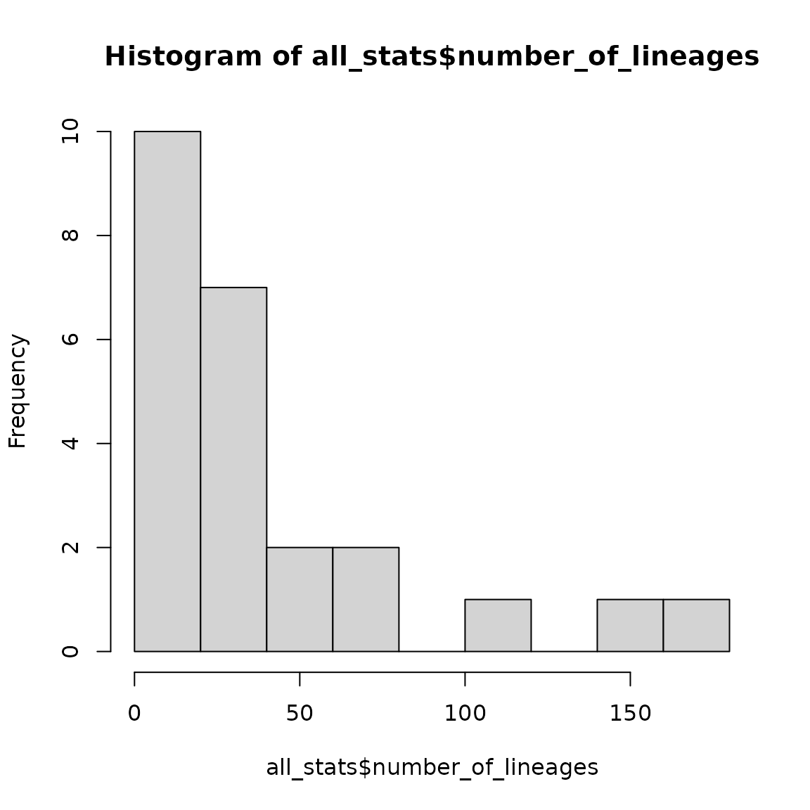

Furthermore, we can make a heatmap of all correlations:

cor.dist <- cor(all_stats)
diag(cor.dist) <- 0
heatmap(cor.dist)

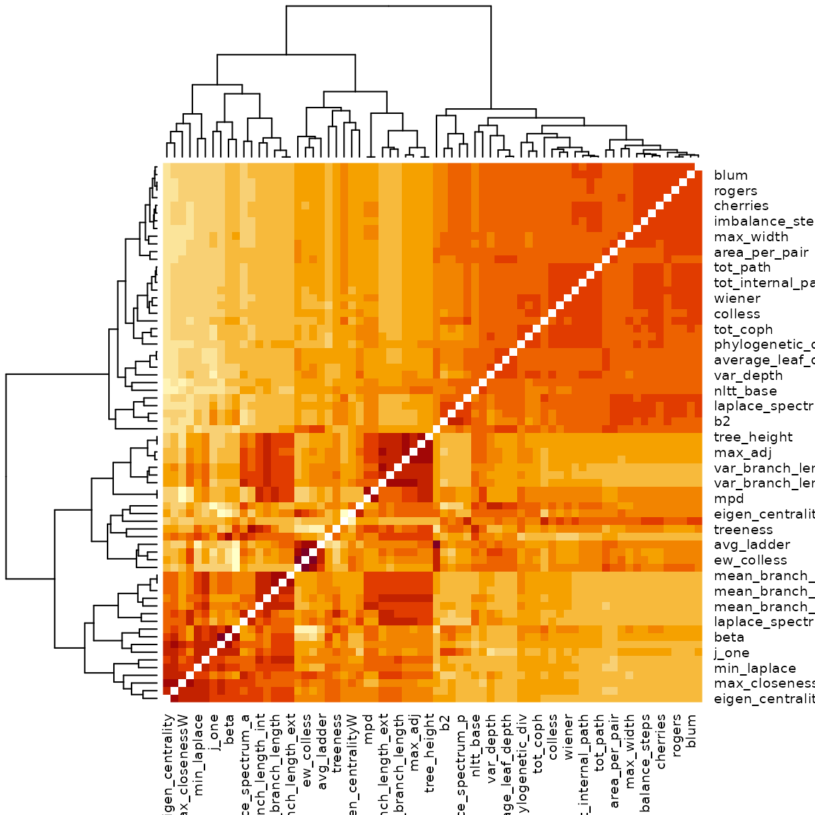
This will generate a distorted image: correlations are not corrected for tree size. We can study this a bit more in detail:

opar <- par()
par(mfrow = c(3, 3))
for (stat in c("area_per_pair", "colless", "eigen_centrality",
               "four_prong", "max_betweenness", "max_width",
               "mntd", "sackin", "wiener")) {
  if (stat != "number_of_lineages") {
    x <- all_stats[, colnames(all_stats) == "number_of_lineages"]
    y <- all_stats[, colnames(all_stats) == stat]
    plot(y ~ x, xlab = "Tree size", ylab = stat, pch = 16)
  }
}

par(opar)

## Warning in par(opar): graphical parameter "cin" cannot be set

## Warning in par(opar): graphical parameter "cra" cannot be set

## Warning in par(opar): graphical parameter "csi" cannot be set

## Warning in par(opar): graphical parameter "cxy" cannot be set

## Warning in par(opar): graphical parameter "din" cannot be set

## Warning in par(opar): graphical parameter "page" cannot be set

To correct for this, we will have to go over the entire correlation matrix.

tree_size <- all_stats[, colnames(all_stats) == "number_of_lineages"]

for (i in seq_len(nrow(cor.dist))) {
  for (j in seq_len(ncol(cor.dist))) {
    stat1 <- rownames(cor.dist)[i]
    stat2 <- colnames(cor.dist)[j]
    x <- all_stats[, colnames(all_stats) == stat1]
    y <- all_stats[, colnames(all_stats) == stat2]

    a1 <- lm(x ~ tree_size)
    a2 <- lm(y ~ tree_size)
    new_cor <- cor(a1$residuals, a2$residuals)
    cor.dist[i, j] <- new_cor
  }
}
diag(cor.dist) <- 0
heatmap(cor.dist)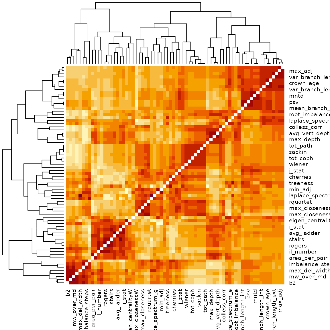

A nicer way to visualize this is given by the package ppheatmap:

if (requireNamespace("pheatmap")) pheatmap::pheatmap(cor.dist)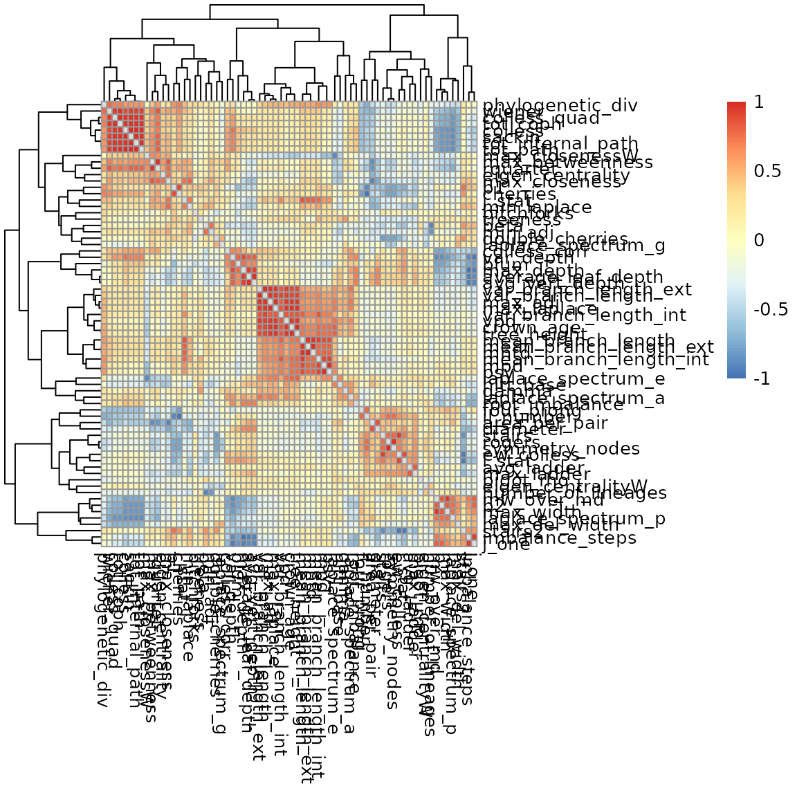

Adding a random category to our matrix

To test whether outliers are perhaps instead of identifying unique information, picking up on random noise, we can also add an extra statistic that has no meaning, and that has random correlations with all other statistics:

cor.dist2 <- cor.dist
rand_values <- runif(n = nrow(cor.dist2))
cor.dist2 <- cbind(cor.dist2, rand_values)
cor.dist2 <- rbind(cor.dist2, c(rand_values, 0))
colnames(cor.dist2)[ncol(cor.dist2)] <- "random"
rownames(cor.dist2)[nrow(cor.dist2)] <- "random"

# and now we plot again:
heatmap(cor.dist2)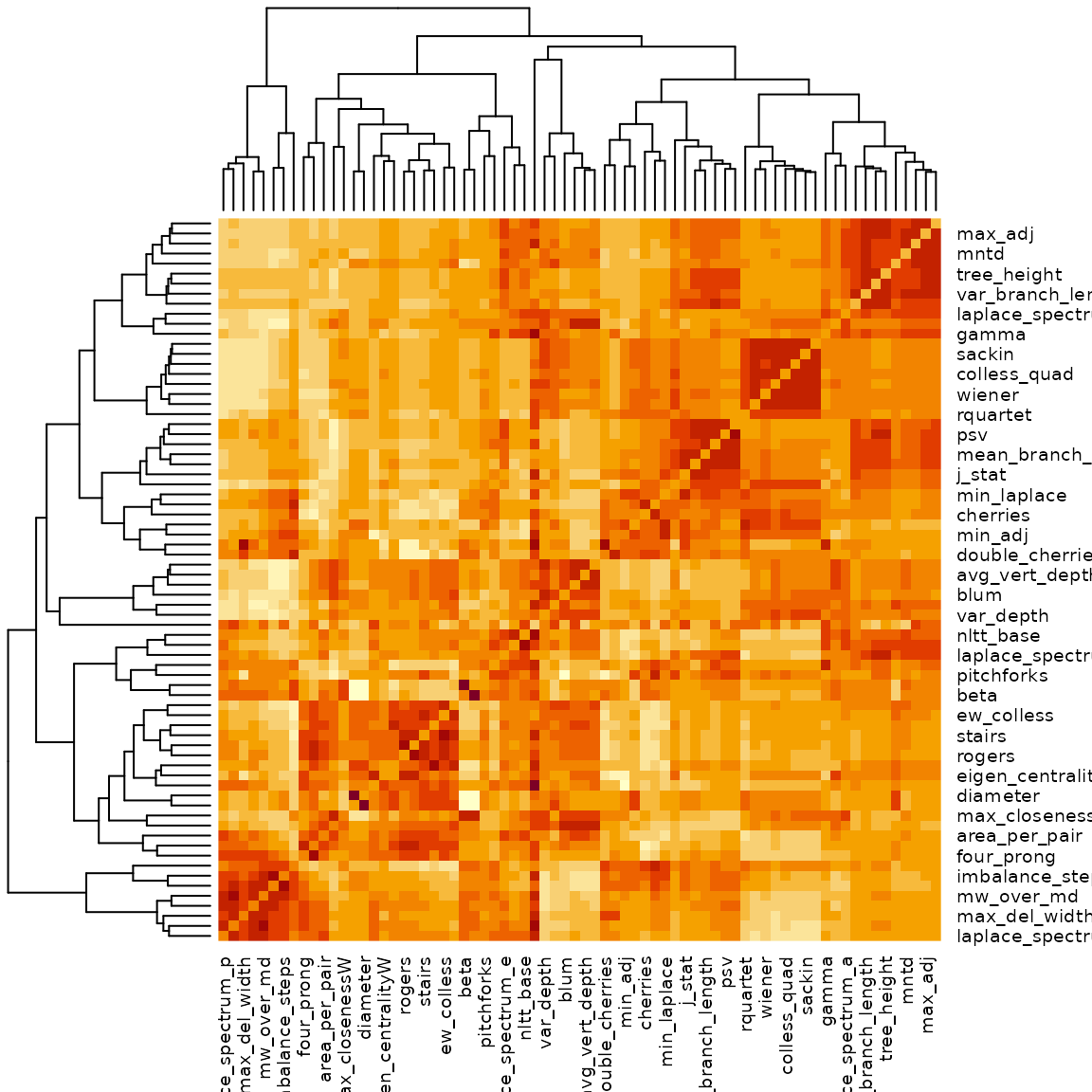

if (requireNamespace("pheatmap")) pheatmap::pheatmap(cor.dist2)

Thijs Janzen

2026-02-27

Data

Adding a random category to our matrix